
Solving the Mystery of Backpropagation
The algorithm is quite the workhorse in the majority of widely used, human-level surpassing learning systems based on neural networks. It…


The algorithm is quite the workhorse in the majority of widely used, human-level surpassing learning systems based on neural networks. It was popularised by the 1986 paper published in Nature authored by David Rumelhart, Geoffrey Hinton, and Ronald Williams.
The original paper concludes, “applying the procedure to various tasks shows that interesting internal representations can be constructed by gradient descent in weight-space, and this suggests that it is worth looking for more biologically plausible ways of doing gradient descent in neural networks”. Well, backpropagation might not exactly be what’s happening in our natural neuron networks, but it surely presented great results in mathematical learning systems. And this would give birth to an exciting new era of Artificial Intelligence.
Backpropagation algorithm deals with a systematic method of continuously adjusting the internal parameters (weights and biases) of a neural network so that the error in the predictions made by the network will be minimum. Understanding of the inside workings of it seems vital if you are looking to work with complex applications of machine learning and deep learning.
The most clever thing about backpropagation seems to be the method used to calculate the partial derivatives of the cost function with respect to each weight and bias in the network. This paves the way to ponder even how this elegant algorithm was found for the first time.
But if you carefully look at the behaviour of the neural network, there might be a systematic way of deducing the mystery of the derivatives.
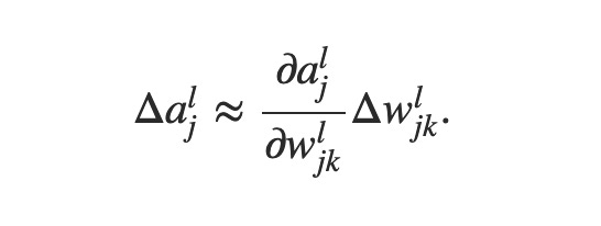
Imagine the case of changing a single weight w value by a small factor Δw as shown below;

Now this change will affect the immediate activation involving that weight, changing it by Δa.

The change of Δa will in-turn affect all the other nodes in the following layer.

And ultimately, passing through all the layers in a similar manner, Δw that started this entire change affects the final cost function.

Now, this we can think of it as a forward propagation of change. In other terms, we can represent the final change in the cost of the network in terms of the first change in weights we manipulated.

Now calculating this change in cost looks like a task of figuring out this term 𝜕C/𝜕w. And looking at how it has been propagated over the network, we can formulate it with respect to all the changes that took place after the first Δw.
The above expression shows the change in the most immediate activation due to Δw. And this will, in turn, affect the next activations following Δa.

Now here Δa can be replaced by the previous expression and you will get the expression below;

We tend to see a pattern arising here. Starting from the first change in Δw, the following activations are affected by the change of activations of the previous layer. ∂a/∂a begins to be a common term to every node we pass through. Now it's clear that for every node in every layer the pattern will prevail as below;

The m, n, p… terms here denote the different layers and the ∑ denotes that we sum over all the node in each layer.
As as we recall the backpropagation algorithm is tasked with finding the partial derivatives of all the parameters, i.e. all the weights and biases with respect to the change in cost at the end of the network. So if we simplify the above equation, it suggests that we can formulate expressions for all the weights and biases in terms of the values of activations and weights. And this procedure of calculating the magnitude of change in every parameter, giving us a direction to follow if we want to reduce the entire magnitude of the cost in the network. The derivatives calculated gives the direction for the gradient descent. Pretty intuitive and elegant.
Now, is this how David Rumelhart et. al. came up with the solution for backpropagation? Well, maybe. But the most fascinating thing about this algorithm is that how these procedures of consistently adapting to the change in cost eventually result in a parameter space that emulates the representation of input data so that it could predict/identify new instances of the same distribution.
This fact is often seen as the mystery of backpropagation, that had made critiques to call deep neural networks a black box. But are they really?
My argument is that if we systematically assess and take time to actually think about what happens during an optimisation period of a neural network, maybe we might be able to wrap our heads around it. But the many levels and levels of abstraction seems to be too much sometimes for our short term memory to withhold and formulate an overall picture of the entire process. And this is what machines are helping us to do.
My closing thoughts are, is this the best that we could come up with though? Because if you think about it, the whole process of generalisation through backpropagation is a very data-hungry and time-consuming process. Will there be more optimum ways for machines to obtain a representation of the objects of the real world? Well, these questions are right at the frontier of research. And we have never been more excited to work on them.
The ideas presented in the post are directly influenced by the book “Neural Networks and Deep Learning” by Michael A. Nielsen. Highly recommended for anyone who wants to learn deep learning from scratch.
Thanks for reading.